


A Deep Dive into Desmoothing and Interpolation Features for Private Assets
Public and private markets are driven by common economic drivers such as economic growth, interest rates, commodities, and credit, which are captured by the factor lens. When the global economy slows, liquid assets such as public equity, and illiquid assets such as private equity, should fall together. However, reported private manager returns often provide a different and unintuitive outcome.
In public markets, investors typically utilize performance that is marked-to-market, in real-time, and daily. On the other hand, private market performance is typically smoothed, marked-to-value, lagged relative to public markets, and infrequent. Smoothed private asset returns may also artificially lower volatility and reduce the explainability of risk, the latter being an important and often overlooked consequence of smoothing. For investors looking to holistically analyze a portfolio that includes private assets, especially alongside public market investments, this data limitation poses a significant hurdle.
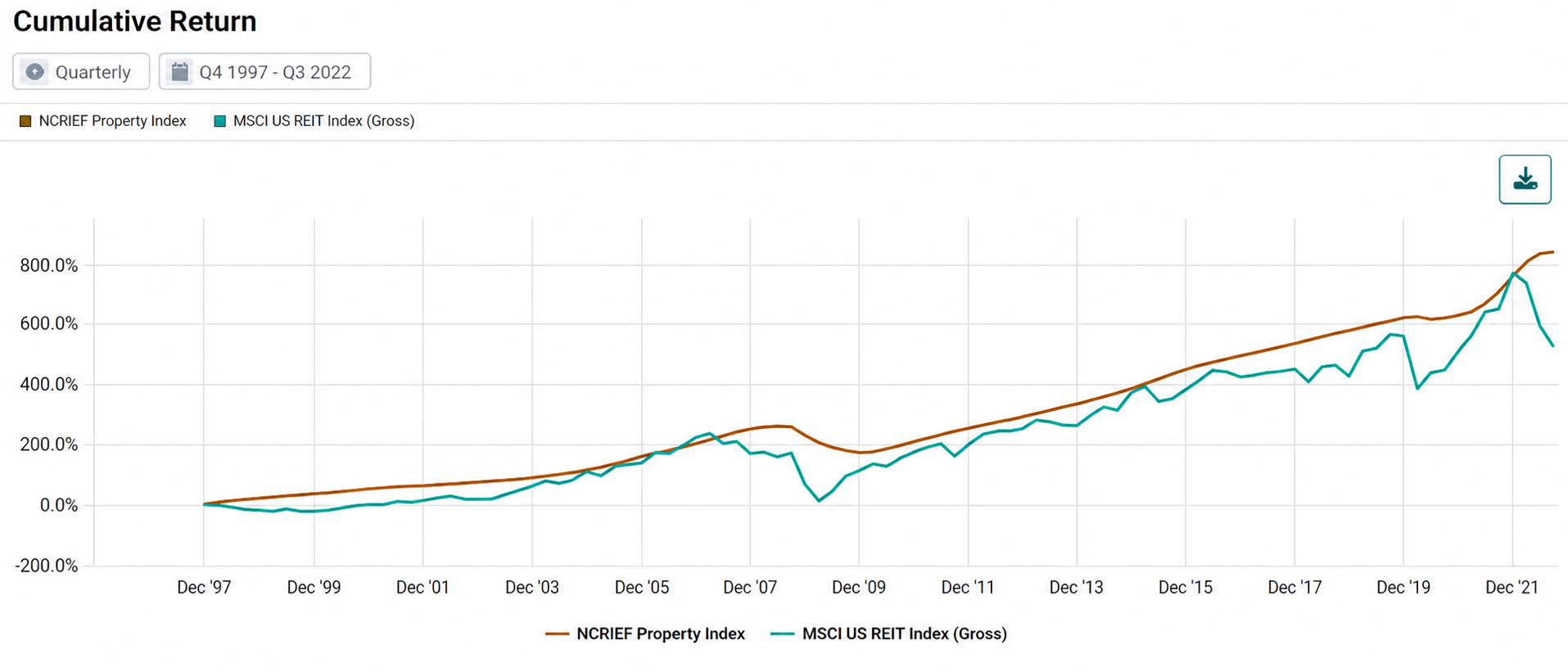
Take a classic private real estate example such as the NCREIF Property index and a public proxy.1 Focusing on the 2009 rebound, private real estate began an upward movement multiple quarters after that of the public proxy, despite being driven by the same common risk factors, such as economic growth and interest rates.
Exhibit 1: Smoothed Private Real Estate Has Lagged Public Markets
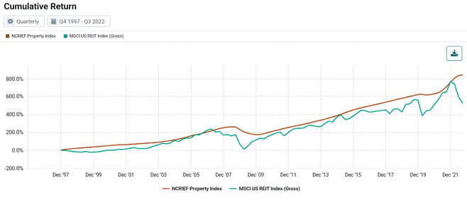
Source: Solovis, Bloomberg. Period from Q4 1997 to Q3 2022. The NCREIF Property index represents private real estate while the MSCI US REIT index represents the public proxy.
Additionally, over this period the private real estate index exhibited a volatility of just 4.42% while the public proxy’s volatility was 21.13%. Understanding that these differences are not likely real, but rather the outcome of smoothed and infrequent private data, promotes a call to action.
How to View Private Asset Data Through a Public Lens
Public market data is frequent and marked to market. As a result, one way to potentially improve the quality of private asset returns is by making them look and feel more like a public market proxy. To accomplish this goal, Solovis Risk Pro applies two statistical methods: desmoothing and interpolation.
Below you can see the role that each method plays on the journey to viewing private asset returns with a public lens. Specifically, desmoothing aims to reduce private market performance lag and mark it to the market, while interpolation aims to increase the frequency of data.
Exhibit 2: Utilizing Desmoothing and Interpolation to Take a Public View
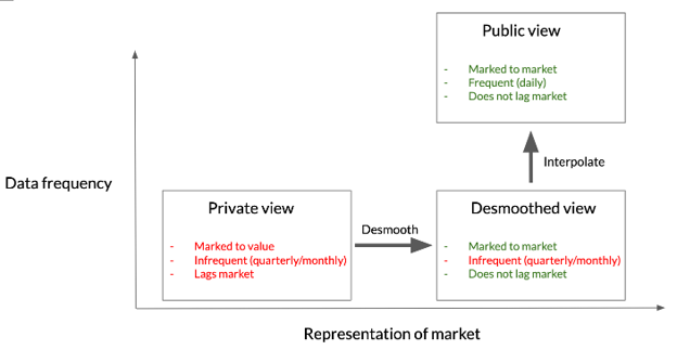
Source: Solovis. For illustration purposes only.
More About Desmoothing
A primary goal of desmoothing is to account for the lag that is typically exhibited between private and public markets. One reason for this lag is that private managers, who are marking their assets to valuation rather than market transactions, typically reveal those asset valuations on a delayed basis.
Risk Pro applies desmoothing to private asset returns following the econometric model by Getmansky, Lo, and Makarov (2004). Put simply, this approach reverse-engineers the smoothing process by examining smoothed private asset performance and its regression-based relationship with an appropriate public proxy.
Three steps best summarize this process:
-
Estimating the relationship of reported returns with public proxy returns
-
Choosing the number of lags to model
-
Reversing the smoothing process
Estimating the Relationship of Reported Returns with Public Proxy Returns
Because a well-chosen public proxy should theoretically be exposed to similar risk factors as the private asset, the public proxy can be used to provide information about how the private asset was smoothed.
To model the relationship between the private asset return and a chosen public proxy, Risk Pro runs multiple regressions using different lagged public proxy return streams. This means running regressions between the private asset return and a public proxy return stream that has been shifted based on the frequency of the private asset (quarterly lags, for example). The private asset should have exposure to both present and past versions of the public proxy, depending on the smoothing profile of the private asset.
The example below shows how different betas (slope) reveal exposure to the public proxy for each lag (more on how to decide on the number of lags later). These betas are aggregated to represent the true economic exposure, then scaled with the aggregated exposure to imply that the information is contained within the selected number of lags. Quantifying this relationship plays a key role in reversing the smoothing process.
Exhibit 3: Estimation Strategy for Private Asset Returns and a Public Proxy
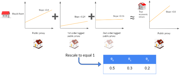
Source: Solovis. For illustrative purposes only.
Choosing the Number of Lags to Model
When estimating the relationship of reported returns with public proxy returns such as those shown in Exhibit 3, the number of lags being used is important. In some cases the investor may know the number of lags that a manager implements when smoothing their returns. In such cases, it will always be best to use the true number of lags as an input to the desmoothing process.
In cases where the number of lags is not known, a statistical process known as Akaike Information Criterion (AIC) can be used. AIC will evaluate multiple models with different numbers of lags, and then select the one of the highest quality. But how many models with different lags should be evaluated? What is the maximum number of lags to allow?
When choosing the number of lags to model through AIC, two assumptions apply:
-
The information will not lag more than 1 year. In the case of quarterly data, there can be more delay, so two extra quarters are allowed to search for lags. Therefore for monthly data: lags ≤ 12 and for quarterly data: lags ≤ 6.
-
There need to be at least 12 observations in the regressions being tested, after considering the number of lags.
Reversing the Smoothing Process
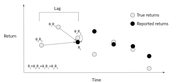
Each theta (Θ), as discussed in Exhibit 3, is treated as a weight in a moving-average model. This means that multiplying each past true return by the corresponding theta should sum to equal the reported return.
Put another way, Θn determines the percent contribution that each past true return plays in the smoothing process to arrive at the reported return to investors. Exhibit 4 illustrates this relationship.
Exhibit 4: Modeling Smoothing Using a Moving Average Process
Source: Solovis. For illustrative purposes only.
Modeling this relationship helps to reverse engineer, or “invert” the smoothing profile and uncover the true economic returns.2
What are some measures of success for a desmoothed return stream?
-
An increase in volatility: Desmoothing returns may increase volatility by adjusting them to more accurately reflect public market volatility.
-
A decrease in autocorrelation: High autocorrelation is a natural bias of smoothing. Decreasing the absolute magnitude of autocorrelation better reflects market reactions (by moving it closer to the autocorrelation of the public proxy) and indicates that past returns are now less similar to future returns.
-
A decrease in residual contribution to risk: The Risk Pro factor lens is designed to be comprehensive, aiming to explain a large degree of portfolio variation. Smoothed private asset returns represent an unnatural market process that leads to larger amounts of unexplainable risk (residual). Desmoothing may reduce this unexplainable risk.
Given these three measures of potential success, the desmoothing process was tested on private real estate, equity, buyouts, and venture capital, with results summarized in Exhibit 5. In every instance, changes in all three measures met expectations: volatility increased, and autocorrelation and residual risk contribution decreased.
Exhibit 5: Results From Desmoothing Various Private Asset Indexes
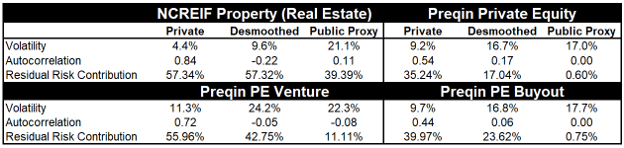
Source: Solovis, Bloomberg. Real Estate analysis from Dec 1997 to Sep 2022. All other analysis from March 2001 to March 2022. Public proxies are based on Preqin’s Public Market Equivalent “Pro Tips” and are as follows: Real Estate: MSCI US REIT index (4 lags used). Private Equity: S&P 500 index (4 lags used). PE Buyout: Russell 3000 index (4 lags used). PE Venture Capital: Russell 2000 index (5 lags used).
Returning to the example from Exhibit 1, the output of the desmoothing feature on the private real estate time series is shown below. Notice how the orange line now rebounds at the same time as the public proxy in 2009.
Exhibit 6: Results from Desmoothing on Private Real Estate
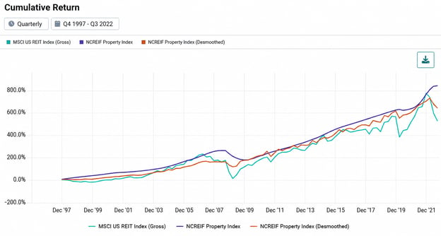
Source: Solovis, Bloomberg. Period from Q4 1997 to Q3 2022. 4 lags used for desmoothing.
More About Interpolation
Despite the illustrated success of the desmoothing results, increasing the frequency of private asset returns is a separate task. Especially when considering consistency across data sets, it can be useful for allocators to convert their quarterly private assets returns into daily.
When interpolating, Risk Pro:
-
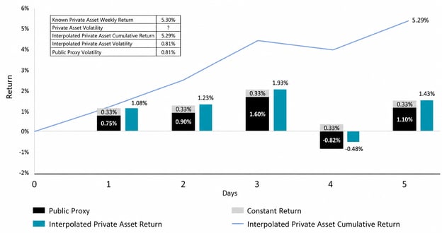
Adds a constant daily return to the chosen public proxy, such that taking the cumulative return should closely match the private asset’s return. That new daily return stream is then used for the private asset. The illustrative example below shows interpolation over a one-week period.
Exhibit 7: Illustrative Example of Interpolation Over One Week
Source: Solovis. For illustration purposes only.
The resulting daily return series approximates that of the original private asset’s return, with a volatility that roughly matches the chosen public proxy.
Exhibit 8 shows the output of both desmoothing and interpolation on private real estate. Notice how this once smoothed quarterly time series now experiences market timing in-line with the public proxy from desmoothing, along with daily volatility incorporated from interpolation.
Exhibit 8: Results from Desmoothing and Interpolation on Private Real Estate
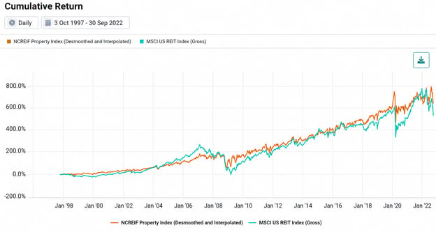
Source: Solovis, Bloomberg. Period from 10/3/1997 to 9/30/2022. 4 lags used for desmoothing
(De)Smoother Sailing When It Comes to Private Asset Returns
Applying the Risk Pro desmoothing approach to private asset returns yields higher volatility while decreasing autocorrelation and residual risk contribution. Additionally, interpolation transforms infrequent data into daily data.
Institutional investors conducting multi-asset portfolio analytics can apply these features to view private assets with a familiar public lens. This may allow investors to better understand levels, timing, and drivers of risk, and may improve operational logistics when working with other daily holdings in the context of a multi-asset portfolio. For portfolio analytics that include private asset returns, these two steps provide a unified public lens.
Contact Solovis to learn more or request a demo.
References:
1Getmansky, Mila, Andrew W. Lo, and Igor Makarov. "An econometric model of serial correlation and illiquidity in hedge fund returns." Journal of Financial Economics 74.3 (2004): 529-609.
2Hamilton, James Douglas (1994). Time Series Analysis. Princeton University Press. ISBN 0-691-04289-6.